The Solution to Binary Classification Task Using XGboost Machine Learning Package

In real life, we quite often come across a class of tasks, where the object of prediction is a nominative variable with 2 gradations, and we need to predict a result of some event or take a decision in binary expression based on data model. For example, if we estimate a situation on the market and our aim is to take a definite decision, whether it makes sense to invest in a certain instrument or not, will a debtor pay off a creditor, or will an employee leave a company soon, etc.

In general, binary classification is applied to predict the probability of happening of a certain event by analyzing a number of features. For this purpose, the so-called dependent variable is introduced (an outcome of an event), which can take only one of two values (which can also be called features, predictors or repressors).

I should make it clear that there are several linear functions in “R” for solving such tasks as “glm” in the standard package of functions, but here we will examine the more advanced variant of binary classification, which is implemented in “XGboost” package. This model, a frequent winner of Kaggle competitions, is based on building binary decision trees, and can support multithreading. The information on the implementation of the family of models “Gradient Boosting” can be found here:

Gradient boosting machines, a tutorial
Gradient boosting (Wikipedia)

Let us take a test dataset (Train) and build a model to predict a number of survivors among passengers in a crash:

    data(agaricus.train, package='xgboost')
    data(agaricus.test, package='xgboost')
    train <- agaricus.train
    test <- agaricus.test

If after transformation the matrix contains a lot of nulls, then such data array should be preliminarily transformed into sparse matrix — in such a case data will take much less space, and, consequently, the time required for data processing will be considerably reduced. At this point, ‘Matrix’ library will come in handy; its last currently available version 1.2-6 contains a set of functions for transformation into dgCMatrix based on columns. In cases, when after all the transformations, already sparse matrix doesn’t fit into random-access memory, a special programme “Vowpal Wabbit” is used. It’s an external programme, which can process datasets of any size, reading from many files or databases.  “Vowpal Wabbit” is an optimized platform for parallel machine learning, developed for distributed computing by “Yahoo!”. You can read about it in detail clicking on this link:

Vowpal Wabbit (Wikipedia)

Usage of sparse matrixes enables us to build a model, using text variables with their preliminary transformation.

Thus, in order to build a matrix of predictors, we should first download the required libraries:

    library(xgboost)
    library(Matrix)
    library(DiagrammeR)

While converting into matrix, all the categorical variables will be transposed; consequently, a function with a standard booster will include their values into a model. The first thing to do is to remove from a data set variables with unique values, such as Passenger ID”, “Name” and “Ticket Number”. Then we do the same with the text data set, which will be used for calculation of predictions of outcomes. For illustration purposes, I loaded the data from local files that I downloaded into the corresponding Kaggle dataset. For the model, we will need the following table columns:

    input.train <- train[, c(3,5,6,7,8,10,11,12)]
    input.test <-  test[, c(2,4,5,6,7,9,10,11)]

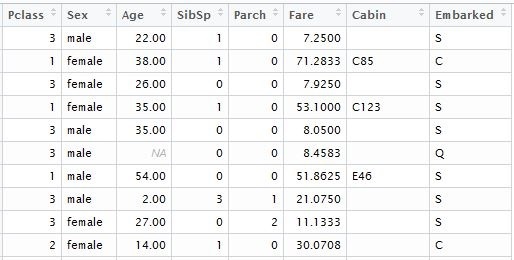
we separately form the vector of known outcomes for model training:

    train.lable <- train$Survived

Now it is necessary to perform data transformation for statistically significant variables to be taken into account. Let us make the following transformations:

Let us replace the variables that contain categorical data with numeric values. At the same time, it should be taken into account that ordered categories, such as “good”, “normal”, “bad”, can be replaced with 0,1,2. Data with relatively small selectivity, such as “gender” or “Country Name” can be left as factorial without any changes; after transformation into matrix, they will transpose into a corresponding number of columns with zeros and ones. For numeric variables, it is necessary to process all the unassigned and missing values. There are at least 3 variants here: they can be replaced with 1,0 or, which is a more acceptable variant, they can be replaced with the average value of the column of this variable.

While using “XGboost” package with a standard booster (gbtree), variable scaling can be omitted, in contrast to other linear methods, such as “glm” or  “xgboost” with linear booster (gblinear).

The main information about the package can be found by clicking on the following links:

xgboost (GitHub)
Package ‘xgboost’ (PDF)

Getting back to our code, as a result, we received a table in the following format:

then we need to replace all the missing notes with the arithmetical average of predictor column:

    if (class;(inp.column) %in %c('numeric', 'integer')) {
        inp.table[is.na(inp.column), i] <- mean(inp.column, na.rm=TRUE)

after pre-processing we need to make a transformation into “dgCMatrix”:

sparse.model.matrix(~., inp.table)

It makes sense to create a separate function for pre-processing of predictors and transformation into sparse.model.matrix format, the version with cycle “for”, for example, is given below.  In order to optimize performance you can vectorize the expression using function “apply”.

    spr.matrix.conversion <- function(inp.table) {
        for (i in 1:ncol(inp.table)) {
            inp.column <- inp.table [ ,i]
            if (class(inp.column) ==         'character') {
                inp.table [is.na(inp.column), i] <- 'NA'
                inp.table [, i] <- as.factor(inp.table [, i])
            }
            else
                if (class(inp.column) %in% c('numeric', 'integer')) {
                    inp.table [is.na(inp.column), i] <- mean(inp.column, na.rm=TRUE)
                }
        }
    return(sparse.model.matrix(~.,inp.table))
    }

Then we will use our function and transform factual and text tables into sparse matrices:

    sparse.train <- preprocess(train)
    sparse.test <- preprocess(test)

To build this model we need 2 datasets: data matrix that we have just created, and

a vector of actual outcomes with a binary value (0,1).

“Xgboost” function is the most user-friendly one. In “XGBoost” a standard booster is implemented, which is based on binary decision trees.

To use “XGboost”, we need to choose one of 3 parameters: general parameters, booster parameters, and purpose parameters:

• General parameters – we define which booster will be used, either linear or standard.
• Other parameters will depend on which booster was chosen at the first step:
• Parameters of learning task – we define the purpose and scenario of learning
• Parameters of command line – they are used to determine the mode of a command line using “xgboost.”.

The general form of “xgboost” function that we use:

    xgboost(data = NULL, label = NULL, missing = NULL, params = list(), nrounds, verbose = 1, print.every.n = 1L, early.stop.round = NULL, maximize = NULL, ...)

“data” – matrix format data ( “matrix”, “dgCMatrix”, local data file or “xgb.DMatrix”)

“label” – vector of dependant variable. If a given field was a part of a source table of parameters, then it should be excluded before processing and transformation into matrix in order to avoid transitivity of connections.

“nrounds” – the number of decision trees in the final model.

“objective” – through this parameter we transfer the tasks and the learning purpose of a model.

“reg:logistic” – logistic regression with a binary value of prediction.

For this parameter, we can set a certain limiting value from 0 to 1. By default, this value is 0.5.

You can read about the parametrization of a model by clicking on this link:

XGBoost Parameters

Now let us proceed to the creation and training of “XGBoost” model:

    set.seed(1)
    xgb.model <- xgboost(data=sparse.train, label=train$Survived, nrounds=100, objective='reg:logistic')

If desired, it is possible to derive the structure of trees with the help of xgb.model.dt.tree( model = xgb) function. Then we should use the standard function “predict” to form the prediction vector:

    prediction <- predict(xgb.model, sparse.test)

And finally, we need to save data in a legible format:

    solution <- data.frame(prediction = round(prediction, digits = 0), test)
    write.csv(solution, 'solution.csv', row.names=FALSE, quote=FALSE)

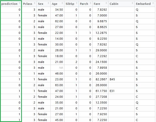
Adding the vector of predicted outcomes, we will get the following table:

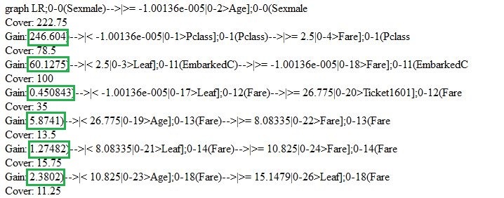
Let us go back and briefly review the model that we have just created. We can use “xgb.model.dt.tree” and “xgb.plot.tree” functions to show decision trees. For instance, the last function will give us the list of chosen trees with the coefficient of model fitting:

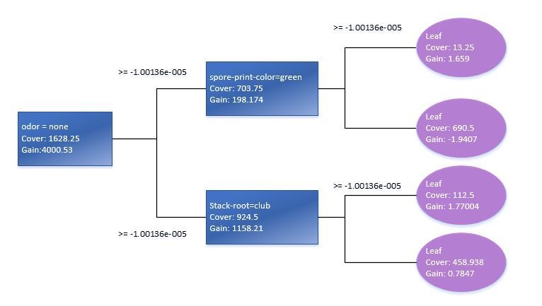
Using xgb.plot.tree function, we will also see the graph representation of trees. It should be pointed out, though, that in the current version it is not implemented in the best way and is of little use. That is why to illustrate this I had to reproduce the basic decision tree manually based on Train standard data model.

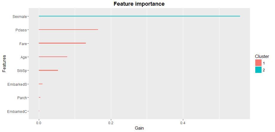
The check of statistical significance of variables in a model will tell us how to optimize the matrix of predictors for XGB-model learning. It is best to use xgb.plot.importance function, in which we will transmit the aggregated table of importance of parameters.

    importance_frame <- xgb.importance(sparse.train@Dimnames[[2]],  model = xgb)
    xgb.plot.importance(importance_frame)

So, we have reviewed one of the possible implementations of logistic regression based on the package of “xgboost” function with a standard booster. I recommend using “XGboost” package as it is by far the most advanced group of machine learning models. Currently, predictive models on the basis of “XGboost” logic are widely used in financial and market forecasting, marketing and many other fields of applied analytics and machine intelligence.